Large scale de-identification is not just a model problem. The hard part is turning model predictions into a reliable service: validate requests, preserve offsets, split long records safely, keep the GPU busy, return useful spans, and make deployment repeatable enough that the system can be operated.
This project started from a Dutch clinical de-identification model and grew into a production-oriented annotation server. The final shape separates application logic from model execution, supports batch clients such as Spark and Delta pipelines, and exposes the operational hooks needed to run it on GPU infrastructure.
The service boundary
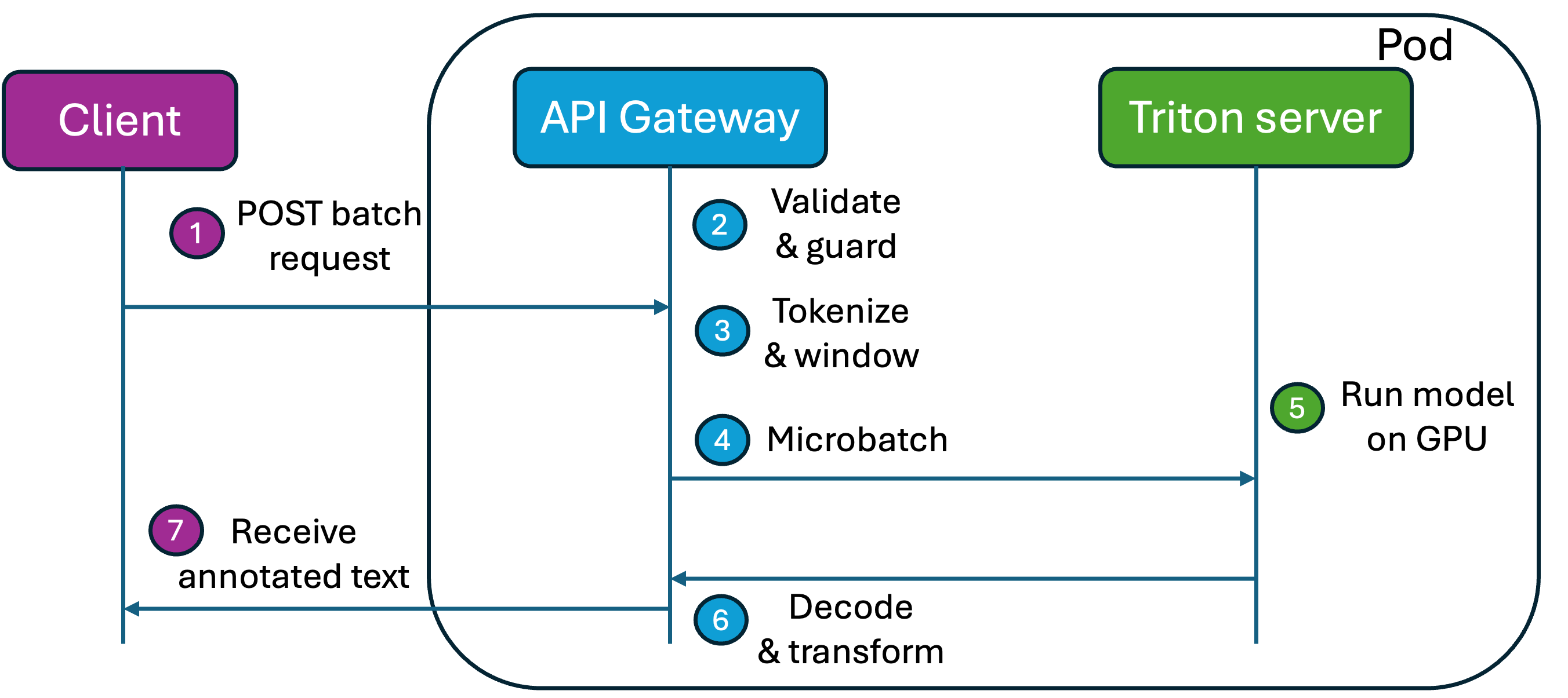
The client sends a batch de-identification request with one or more text records, optional metadata, and processing options. The API Gateway validates the schema and enforces safety limits before doing any expensive work: request bytes, record count, characters per record, characters per request, and maximum model windows.
After validation, the gateway tokenizes each record and splits longer documents into model-sized sliding windows. It keeps the token offsets so predictions can be mapped back to the original character positions. Those windows are grouped into microbatches, padded into input_ids and attention_mask tensors, and sent to the inference runtime.
The Triton server has a deliberately small job: run the optimized model on the GPU and return raw logits, such as Beginning-Inside-Outside (BIO) logits and entity-label logits. It does not validate API requests, tokenize text, decode spans, or build the final response. Once the logits return, the gateway averages overlapping window predictions, decodes BIO tags into personally identifiable information (PII) spans, maps spans back to the source text, applies post-processing, handles date replacement, and returns the de-identified records.
That separation was one of the main architectural lessons. The inference server should not become a second application server. It should be a narrow, fast model runtime behind an API layer that understands the product contract.
Throughput depends on the whole path
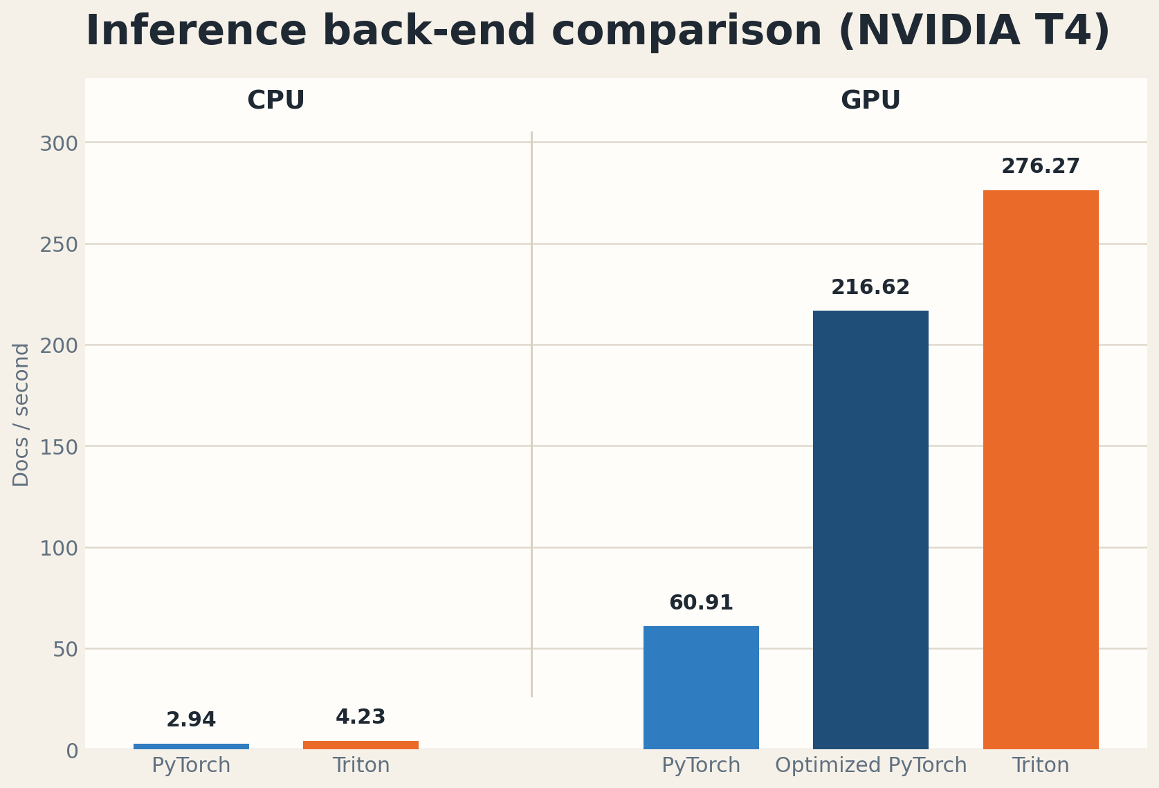
The first benchmark lesson was obvious but important: CPU inference was not a realistic production target for large volumes. In the T4 runs, CPU paths were around 3 to 4 docs/s. Plain CUDA PyTorch moved that to about 61 docs/s. Adding torch.compile with reduce-overhead mode and float16 autocast moved optimized PyTorch to about 217 docs/s.
The fastest result in the consolidated report was about 276 docs/s using the TensorRT model.plan engine on the GPU. Moving from plain model execution to an optimized TensorRT engine changed the throughput envelope from a few documents per second to hundreds.
The second throughput lesson was less obvious: batching policy and request shape mattered as much as the raw backend. The gateway uses microbatching with limits on windows, tokens, wait time, queued windows, and queued requests. The tuned configuration used 16 windows, 4096 tokens, a 5 millisecond (ms) max wait, two Uvicorn workers, and bounded queues. For high-volume offline jobs, packing requests by estimated model windows was better than using a fixed record count, because clinical text length has a long tail.
Scaling was measured, not assumed
The current defaults are not arbitrary. They came from tuning three layers: gateway microbatching, client-side request packing, and Kubernetes serving scale.
At the gateway layer, the best documented T4 setting was 16 windows per microbatch, 4096 tokens per microbatch, a 5 millisecond (ms) maximum wait, and two Uvicorn workers. The two-worker setting helped sustained throughput, while four workers hurt long-text tail latency.
At the Spark/Delta layer, packing by estimated model windows worked better than a fixed record count. The practical target was about 160 windows per request, capped at 64 records and 80,000 characters per request, with a rough window estimate of ceil(chars / 512). This matters because the realistic text distribution had a long tail: short median records, a much higher mean, and records up to roughly 37k characters.
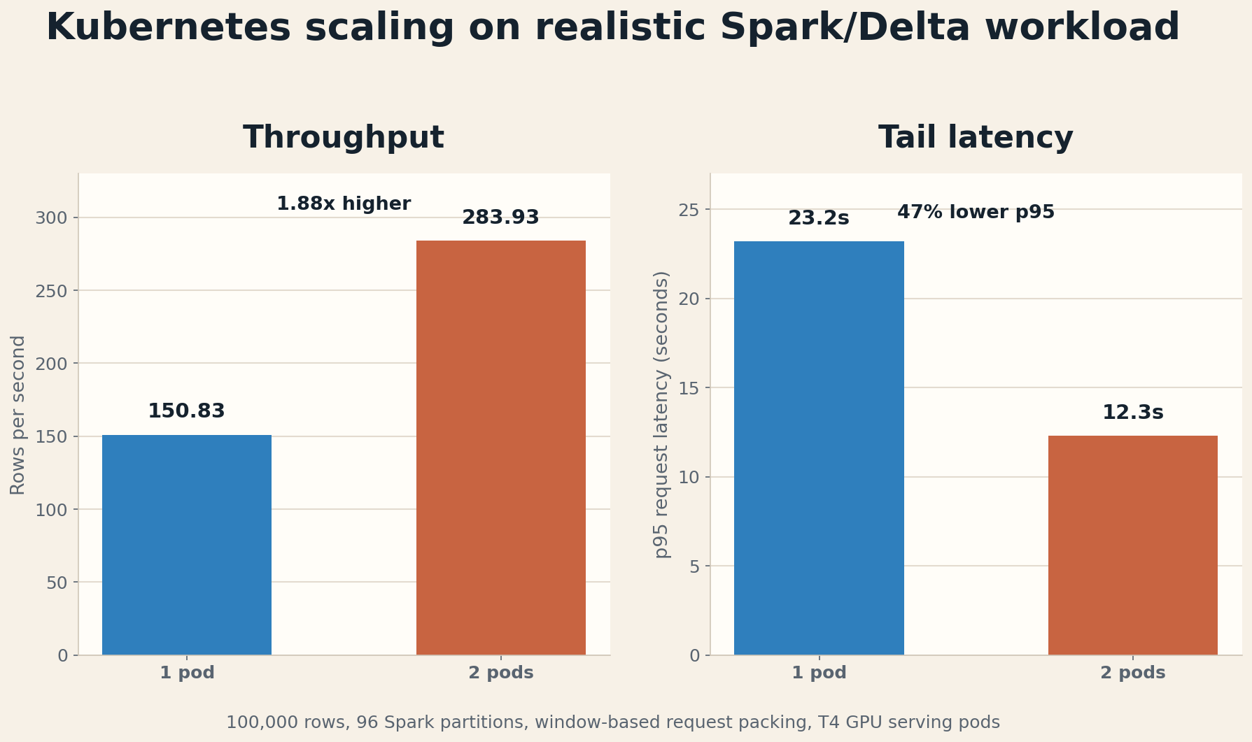
The most important result was the Kubernetes realistic benchmark. On 100,000 rows with 96 source partitions, 96 output partitions, eight requests per partition, and window-based packing, one serving pod handled 150.83 rows/s and 502.38 windows/s. Two serving pods handled 283.93 rows/s and 945.69 windows/s. That is a 1.88x speedup, while p95 request latency dropped from 23.2s to 12.3s.
The absolute p95 latency is still high if this were an interactive API. In this benchmark, though, requests were deliberately packed for offline Spark/Delta throughput: up to about 160 model windows, 64 records, and 80,000 characters per request. So I read the latency as a batch-processing tradeoff, not as the latency target for single-note interactive serving.
The throughput number is consistent with that packing. In the two-pod run, 100,000 rows were processed in 2,193 API requests over 352.2 seconds. That is 6.23 requests/s. Each request contained 45.6 rows on average, so 6.23 * 45.6 = 284 rows/s. The mean request latency was 5.8s, which implies about 6.23 * 5.8 = 36 concurrent in-flight requests. Spark provided that concurrency through its partitions, so high per-request latency and high total throughput can exist at the same time.
The high p95 is also likely related to the long tail of text lengths. Most records were much shorter, but some notes were tens of thousands of characters and expanded into many model windows. Those heavy requests drive tail latency, while the rest of the Spark partitions keep the service busy enough to maintain high overall throughput.
What made it production-grade
The most important work was not one optimization. It was the set of constraints around the model:
- A stable batch JSON API for internal extract, transform, load (ETL) and Spark callers.
- A model bundle contract with label order, window length, overlap, thresholds, and model version metadata.
- Request limits before tokenization and model-window limits after tokenization.
- Sliding windows with overlap, offset tracking, and reconstruction back to character spans.
- A post-processing layer for span cleanup, patient-name recovery from metadata, date shifting, birthdate handling, and replacements.
- Bounded microbatch queues that return overload instead of growing without limit.
- Health, readiness, and Prometheus metrics for request latency, queue wait, batch fill reason, inference time, and overloads.
- Release manifests that keep gateway images and model images paired for rollout and rollback.
Those pieces are what make the service usable beyond a demo. A strong model can still fail operationally if the surrounding harness is not engineered with care.
The bigger lesson
I went into this thinking mostly about serving a de-identification model. I came out thinking about the entire annotation system around it: the API contract, the data pipeline, runtime boundaries, request packing, GPU utilization, deployment artifacts, readiness, and rollback.
For large scale clinical de-identification, the production system is the product. The model is central, but the surrounding engineering determines whether it can safely process real workloads at scale.
If you work in a health organization and want to test this kind of de-identification setup on your own clinical text workflow, send me an email at stig.hellemans@uantwerpen.be.
This work was developed in the context of my research at the University of Antwerp and UZA, within Adrem Data Lab, with support from FWO (1SA3226N).